Note
Click here to download the full example code
Basis functions
In the previous tutorial we have seen that overlapping even-related time courses can be recovered using the general linear model, as long as we assume they add up linearly and are time-invariant.
# Import libraries and setup plotting
from nideconv.utils import double_gamma_with_d
import numpy as np
import matplotlib.pyplot as plt
import seaborn as sns

sns.set_style('white')
sns.set_context('notebook')
Well-specified model
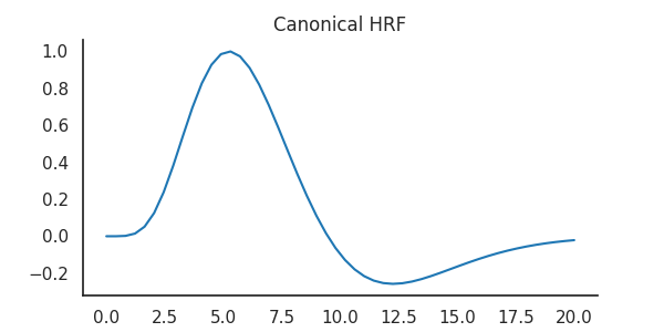
Another important assumption pertains to what we believe the response we are interested in looks like. In the most extreme case, we for example assume that a task-related BOLD fMRI response exactly follows the canonical HRF.
plt.figure(figsize=(6,3))
t = np.linspace(0, 20)
plt.plot(t, double_gamma_with_d(t))
plt.title('Canonical HRF')
sns.despine()
Let’s simulate some data with very little noise and the standard HRF, fit a model, and see how well our model fits the data
from nideconv import simulate
from nideconv import ResponseFitter

conditions = [{'name':'Condition A',
              'mu_group':5,
              'std_group':1,
               'onsets':[0, 20]}]

# Simulate data with very short run time and TR for illustrative purposes
data, onsets, pars = simulate.simulate_fmri_experiment(conditions,
                                                       TR=0.2,
                                                       run_duration=40,
                                                       noise_level=.2,
                                                       n_rois=1)

# Make ResponseFitter-object to fit these data
rf = ResponseFitter(input_signal=data,
                    sample_rate=5) # Sample rate is inverse of TR (1/TR)
rf.add_event('Condition A',
             onsets.loc['Condition A'].onset,
             interval=[0, 20],
             basis_set='canonical_hrf')

rf.fit()

rf.plot_model_fit()
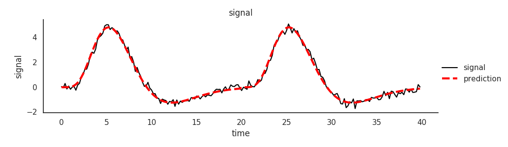
As you can see, the model fits the data well, the model is well-specified.
Mis-specified model
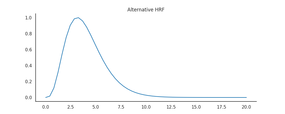
Now let’s what happens with data with different HRF from what the model assumes.
# For this HRF the first peak is much earlier (approx 3.5 seconds versus 5.8)
# and the second "dip" is not there (c=0).
kernel_pars = {'a1':3.5,
               'c':0}

plt.plot(t, double_gamma_with_d(t, **kernel_pars))
plt.title('Alternative HRF')
sns.despine()
plt.gcf().set_size_inches(10, 4)
Simulate data again
data, onsets, pars = simulate.simulate_fmri_experiment(conditions,
                                                       TR=0.2,
                                                       run_duration=50,
                                                       noise_level=.2,
                                                       n_rois=1,
                                                       kernel_pars=kernel_pars)

rf = ResponseFitter(input_signal=data,
                    sample_rate=5)
rf.add_event('Condition A',
             onsets.loc['Condition A'].onset,
             interval=[0, 20],
             basis_set='canonical_hrf')
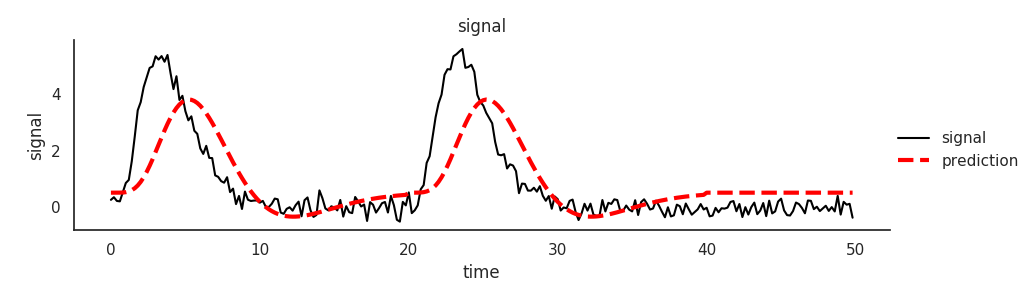
Plot the model fit
rf.fit()
rf.plot_model_fit()
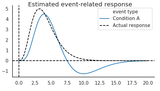
And the estimated time course
def plot_estimated_and_actual_tc(rf,
                                 kernel_pars=kernel_pars,
                                 amplitudes=[5]):
    """
    Plots estimated event-related responses plus the actual underlying
    responses given by kernel_pars and amplitudes
    """
    rf.plot_timecourses(legend=False)
    t = np.linspace(0, 20)

    # Allow for plotting multiple amplitudes
    amplitudes = np.array(amplitudes)
    plt.plot(t,
             double_gamma_with_d(t, **kernel_pars)[:, np.newaxis] * amplitudes,
             label='Actual response',
             ls='--',
             c='k')

    plt.legend()
    plt.suptitle('Estimated event-related response')
    plt.tight_layout()


plot_estimated_and_actual_tc(rf)
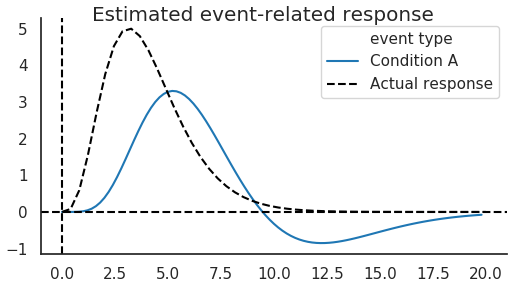
The estimated time-to-peak is completely off
print(rf.get_time_to_peak())
Out:
time to peak
area                             signal
event type  covariate peak
Condition A intercept 1            5.24
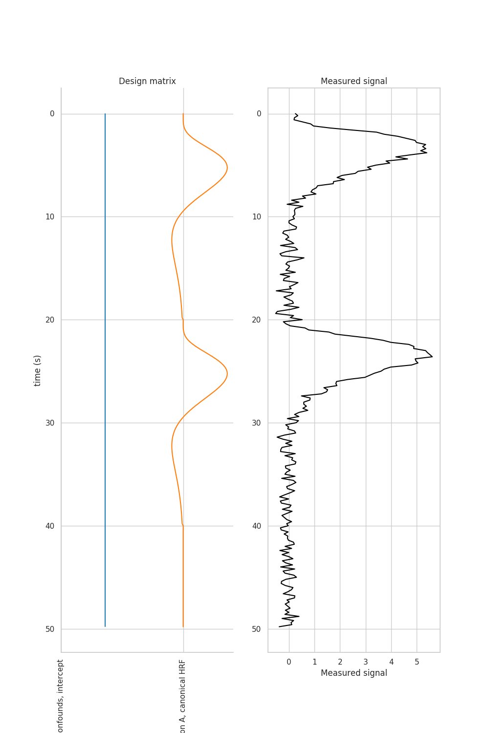
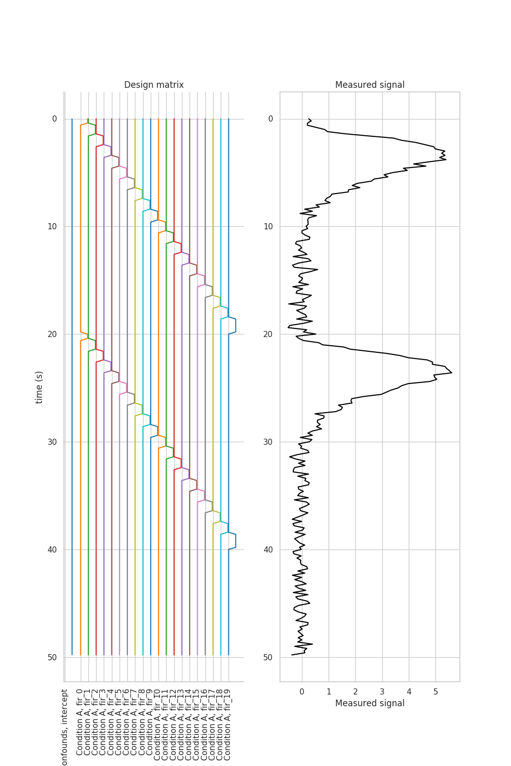
Clearly, the model now does not fit very well. This is because the design matrix \(X\) does not allow for properly modelling the event-related time course. No matter what linear combination \(\beta\) you take of the intercept and canonical HRF (that has been convolved with the event onsets), the data can never be properly explained.
def plot_design_matrix(rf):
    """
    Plots the design matrix of rf in left plot, plus the signal
    it should explain in the right plot.
    Time is in the vertical dimension. Each regressor in X is plotted
    as a seperate line.
    """
    sns.set_style('whitegrid')
    ax = plt.subplot(121)
    rf.plot_design_matrix()

    plt.title('Design matrix')

    plt.subplot(122, sharey=ax)
    plt.plot(rf.input_signal, rf.input_signal.index, c='k')
    plt.title('Measured signal')
    plt.xlabel('Measured signal')

    plt.gcf().set_size_inches(10,15)
    sns.set_style('white')

plot_design_matrix(rf)
The derivative of the cHRF with respect to time
The solution to this mis-specification is to increase the model complexity by adding extra regressors that increase the flexibility of the model. A very standard approach in BOLD fMRI is to include the derivative of the HRF with respect to time for dt=0.1. Then the design matrix looks like this
rf = ResponseFitter(input_signal=data,
                    sample_rate=5)
rf.add_event('Condition A',
             onsets.loc['Condition A'].onset,
             interval=[0, 20],
             basis_set='canonical_hrf_with_time_derivative') # note the more complex
                                                             # basis function set

plot_design_matrix(rf)
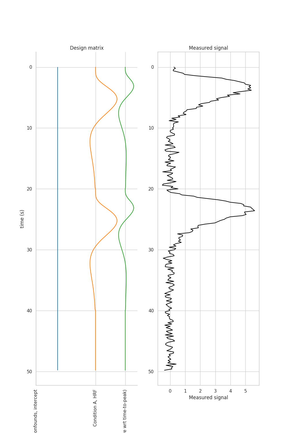
The GLM can now “use the new, red regressor” to somewhat shift the original HRF earlier in time.
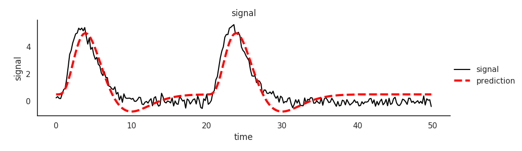
rf.fit()
rf.plot_model_fit()
plot_estimated_and_actual_tc(rf)
The estimated time-to-peak is more in the range of what it should be
print(rf.get_time_to_peak())
Out:
time to peak
area                             signal
event type  covariate peak
Condition A intercept 1            3.89
Even more complex basis functions
Note that the canonical HRF model-with-derivative still does not fit perfectly: the Measured signal is still peaking earlier in time than the model. And the model still assumes as post-peak dip that is not there in the data. Therefore, it also underestimates the height of the first peak.
One solution is to use yet more complex basis functions, such as the Finite Impulse Response functions we used in the previous tutorial. This basis functions consists of one regressor per time-bin (as in time offset since event).
rf = ResponseFitter(input_signal=data,
                    sample_rate=5)
rf.add_event('Condition A',
             onsets.loc['Condition A'].onset,
             interval=[0, 20],
             basis_set='fir',
             n_regressors=20) # One regressor per second

plot_design_matrix(rf)
Clearly, this model is much more flexible, and, hence, it fits better:
rf.fit()
rf.plot_model_fit()
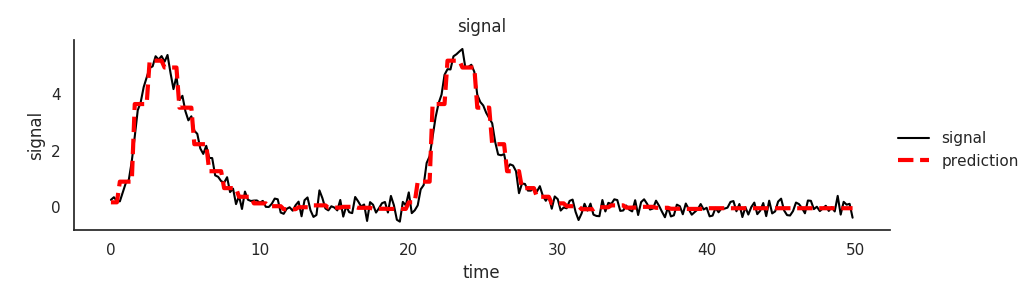
Clearly, this model is much more flexible, and, hence, it fits better:
plot_estimated_and_actual_tc(rf)
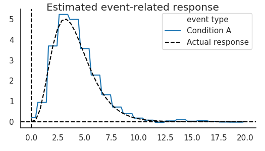
Also, the estimated time-to-peak is more in the range of where it should be
print(rf.get_time_to_peak())
Out:
time to peak
area                             signal
event type  covariate peak
Condition A intercept 1             3.0
No Free Lunch (Bias-Variance tradeoff)
The higher flexibility of the FIR model is due to its higher degrees-of-freedom, roughly the number of regressors. It is important to note that a higher number of degrees-of-freedom also mean a higher variance of the model. A higher variance means that smaller fluctuations in the data will lead to larger differences in parameter estimates. This is especially problematic in high-noise regimes. The following simulation will show this.
Simulation
# Set a random seed so output will always be the same
np.random.seed(666)

# Simulate data
TR = 0.5
sample_rate = 1./TR
data, onsets, pars = simulate.simulate_fmri_experiment(noise_level=2.5,
                                                       TR=TR,
                                                       run_duration=1000,
                                                       n_trials=100,
                                                       kernel_pars=kernel_pars)
# cHRF model
hrf_model = ResponseFitter(data, sample_rate)
hrf_model.add_event('Condition A', onsets.loc['Condition A'].onset, interval=[0, 20], basis_set='canonical_hrf')
hrf_model.add_event('Condition B', onsets.loc['Condition B'].onset, interval=[0, 20], basis_set='canonical_hrf')

# cHRF model with derivative wrt time-to-peak
hrf_dt_model = ResponseFitter(data, sample_rate)
hrf_dt_model.add_event('Condition A', onsets.loc['Condition A'].onset, interval=[0, 20], basis_set='canonical_hrf_with_time_derivative')
hrf_dt_model.add_event('Condition B', onsets.loc['Condition B'].onset, interval=[0, 20], basis_set='canonical_hrf_with_time_derivative')

# FIR_model
fir_model = ResponseFitter(data, sample_rate)
fir_model.add_event('Condition A', onsets.loc['Condition A'].onset, interval=[0, 20])
fir_model.add_event('Condition B', onsets.loc['Condition B'].onset, interval=[0, 20])
Simplest model (cHRF)
hrf_model.fit()
plot_estimated_and_actual_tc(hrf_model,
                             amplitudes=pars.amplitude.tolist())
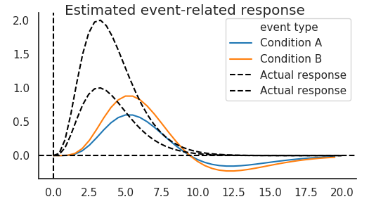
print(hrf_model.get_time_to_peak())
Out:
time to peak
area                             signal
event type  covariate peak
Condition A intercept 1            5.25
Condition B intercept 1            5.25
Extend model (cHRF + deriative wrt time)
hrf_dt_model.fit()
plot_estimated_and_actual_tc(hrf_dt_model,
                             amplitudes=pars.amplitude.tolist())
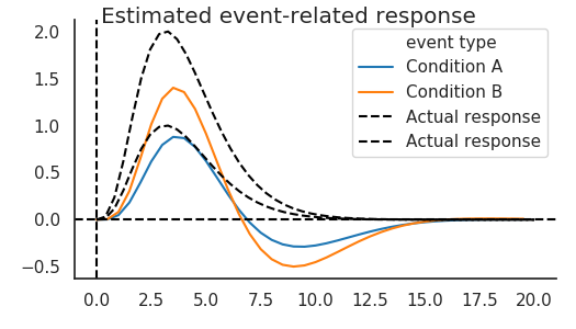
print(hrf_dt_model.get_time_to_peak())
Out:
time to peak
area                             signal
event type  covariate peak
Condition A intercept 1            3.75
Condition B intercept 1            3.65
Most complex model (FIR)
fir_model.fit()
plot_estimated_and_actual_tc(fir_model,
                             amplitudes=pars.amplitude.tolist())
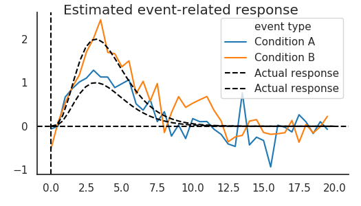
print(fir_model.get_time_to_peak())
Out:
time to peak
area                             signal
event type  covariate peak
Condition A intercept 1             3.0
Condition B intercept 1             3.5
The price of complexity
As you can see, the simplest model does not perform very well, because it is mis-specified to such a large degree. However, the most complex model (FIR) also does not perform very well: the estimated event-related time course is extremely noisy and it looks very “spiky”. The cHRF that includes a derivative wrt to time also doesn’t perform perfectly, because it assume as post-peak undershoot.
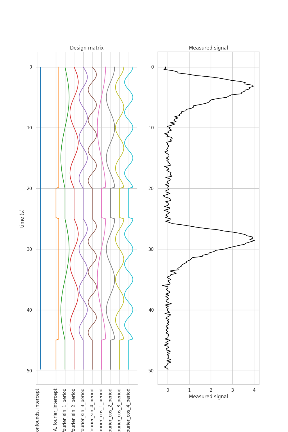
Another basis function set that is quite useful for slow, smooth time courses like fMRI BOLD and the pupil is the Fourier set. It consists of an intercept and sine-cosine pairs of increasing frequency.
conditions = [{'name':'Condition A',
              'mu_group':5,
              'std_group':1,
               'onsets':[0, 25]}]

TR = 0.2
sample_rate = 1./TR

data, onsets, pars = simulate.simulate_fmri_experiment(conditions,
                                                       TR=TR,
                                                       run_duration=50,
                                                       noise_level=.1,
                                                       n_rois=1,
                                                       kernel_pars=kernel_pars)

fourier_model = ResponseFitter(data, sample_rate)
fourier_model.add_event('Condition A',
                        onsets.loc['Condition A'].onset,
                        basis_set='fourier',
                        n_regressors=9,
                        interval=[0, 20])
plot_design_matrix(fourier_model)
fourier_model.fit()
plot_estimated_and_actual_tc(fourier_model,
                             amplitudes=pars.amplitude.tolist())
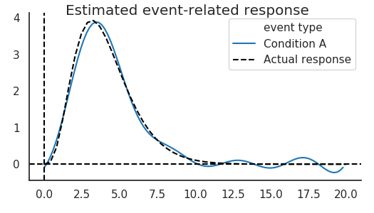
print(rf.get_time_to_peak())
Out:
time to peak
area                             signal
event type  covariate peak
Condition A intercept 1             3.0
Smoothness constraint
The Fourier model combines the flexibility of the FIR model, with a lower number of degrees of freedom. It can do so because the number of time courses it can explain is reduced. It can only account for smooth time courses with lower temporal frequencies. This is a good thing for many applications, like BOLD fMRI, where we know that the time course has to be smooth, since this is the nature of the neurovascular response (a similar argument can be made for pupil dilation time courses).
Conclusion
This tutorial showed how we can use different basis functions in our GLM to deconvolve event-related responses. We can very constrained basis functions, like the canonical HRF, our very flexible basis functions, like the FIR basis set. In general, a balance should be struck between flexibility and degrees of freedom, which can in part be acheived by using basis functions that are targeted towards the kind of responses that are to be expected, notably responses that are temporally smooth. The Fourier basis set is a good example of a generic basis set that allows for relative flexibility with relatively low number of degrees of freedom.
Total running time of the script: ( 0 minutes 11.525 seconds)