Note
Click here to download the full example code
Deconvolution on group of subjects
The GroupResponseFitter-object of Nideconv offers an easy way to fit the data of many subjects together well-specified model nideconv.simulate can simulate data from multiple subjects.
from nideconv import simulate

data, onsets, pars = simulate.simulate_fmri_experiment(n_subjects=8,
                                                       n_rois=2,
                                                       n_runs=2)
Now we have an indexed Dataframe, data, that contains time series for every subject, run, and ROI:
print(data.head())
Out:
area 1    area 2
subject run t
1       1   0.0  0.108141  0.206549
            1.0 -0.199233  0.100078
            2.0  0.152216  1.322024
            3.0 -0.209591  0.410515
            4.0 -1.206617 -0.040518
print(data.tail())
Out:
area 1    area 2
subject run t
8       2   295.0  2.797666  2.103899
            296.0 -0.308147  0.574413
            297.0  0.122700  1.787650
            298.0  1.305447  2.825086
            299.0  1.271533  1.641312
We also have onsets for every subject and run:
print(onsets.head())
Out:
onset
subject run trial_type
1       1   Condition A  219.820716
            Condition A  103.107395
            Condition A  266.262272
            Condition A    7.918901
            Condition A   89.896628
print(onsets.tail())
Out:
onset
subject run trial_type
8       2   Condition B  182.382405
            Condition B  237.654933
            Condition B  258.877295
            Condition B   63.358865
            Condition B   37.917893
We can now use GroupResponseFitter to fit all the subjects with one object:
from nideconv import GroupResponseFitter


# `concatenate_runs` means that we concatenate all the runs of a single subject
# together, so that we have to fit only a single GLM per subject.
# A potential advantage is that the GLM has less degrees-of-freedom
# compared to the amount of data, so that the esitmate are potentially more
# stable.
# A potential downside is that different runs might have different intercepts
# and/or correlation structure.
# Therefore, by default, the `GroupResponseFitter` does _not_ concatenate
# runs.
g_model = GroupResponseFitter(data,
                              onsets,
                              input_sample_rate=1.0,
                              concatenate_runs=False)
We use the add_event-method to add the events we are interested in. The GroupResponseFitter then automatically collects the right onset times from the onsets-object.
We choose here to use the Fourier-basis set, with 9 regressors.
g_model.add_event('Condition A',
                  basis_set='fourier',
                  n_regressors=9,
                  interval=[0, 20])

g_model.add_event('Condition B',
                  basis_set='fourier',
                  n_regressors=9,
                  interval=[0, 20])
We can fit all the subjects at once using the fit-method
g_model.fit()
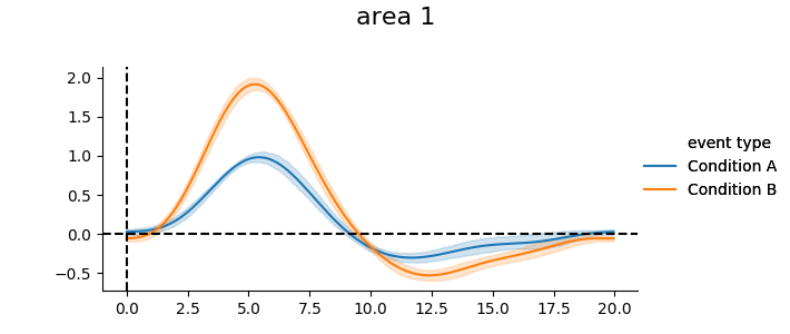
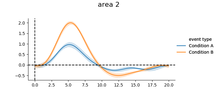
We can plot the mean timecourse across subjects
print(g_model.get_subjectwise_timecourses().head())
g_model.plot_groupwise_timecourses()
Out:
area 1    area 2
subject event type  covariate time
1       Condition A intercept 0.00  0.056636  0.047815
                              0.05  0.056482  0.047954
                              0.10  0.056218  0.047809
                              0.15  0.055854  0.047394
                              0.20  0.055398  0.046727
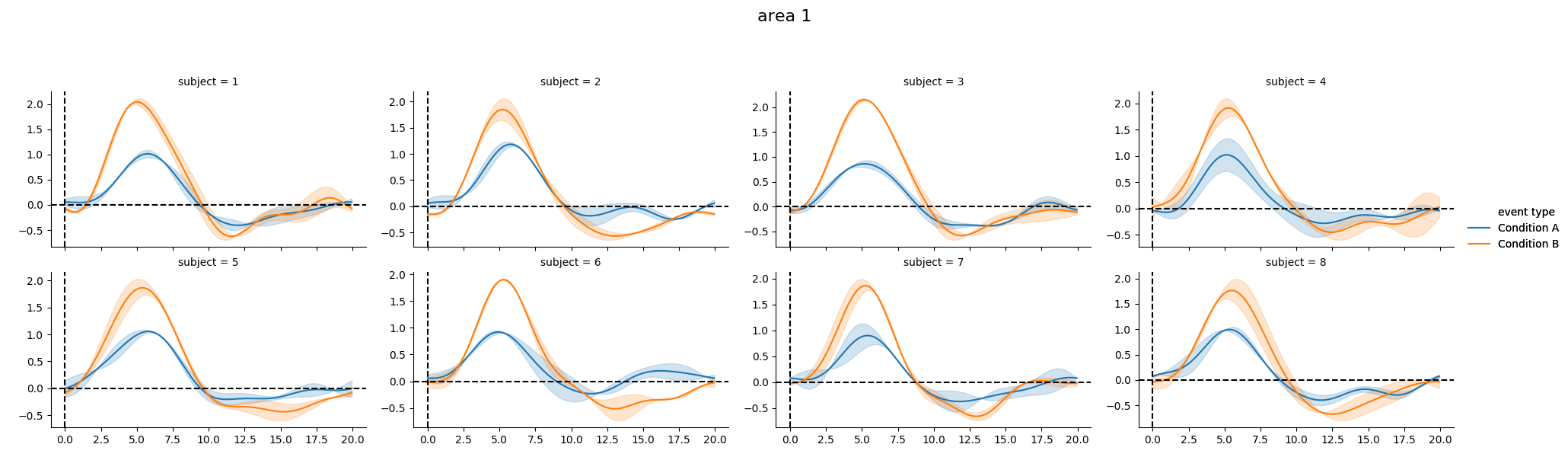
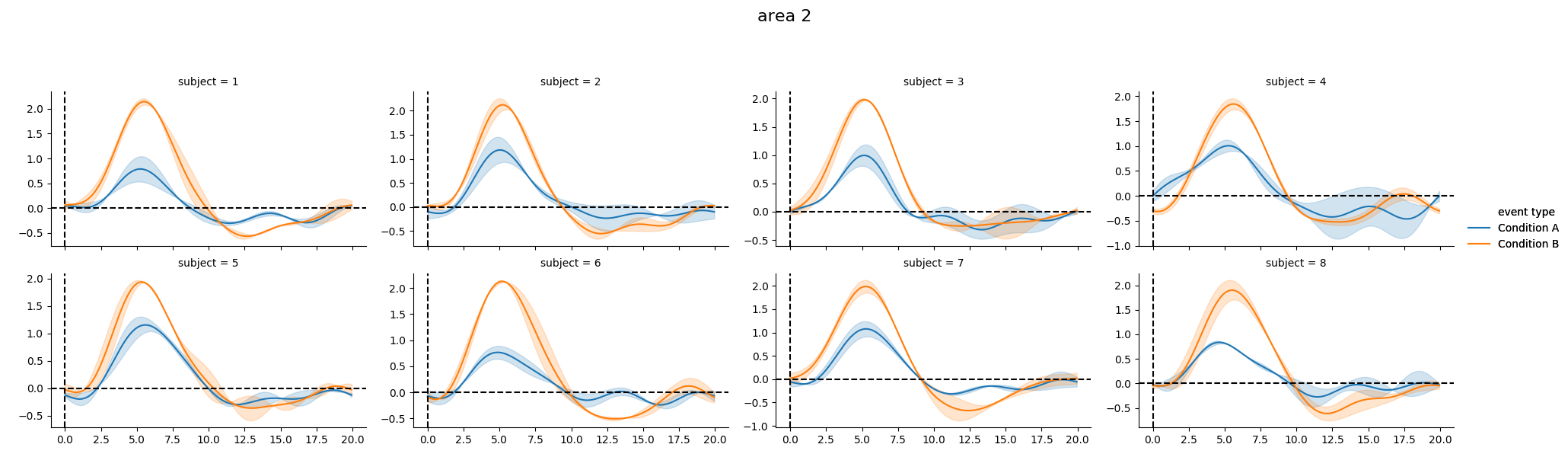
As well as individual time courses
print(g_model.get_conditionwise_timecourses())
g_model.plot_subject_timecourses()
Out:
area 1    area 2
event type  covariate time
Condition A intercept 0.00   0.027545 -0.039614
                      0.05   0.028095 -0.039715
                      0.10   0.028649 -0.039852
                      0.15   0.029217 -0.040009
                      0.20   0.029811 -0.040169
                      0.25   0.030440 -0.040316
                      0.30   0.031117 -0.040429
                      0.35   0.031852 -0.040491
                      0.40   0.032659 -0.040482
                      0.45   0.033549 -0.040383
                      0.50   0.034535 -0.040174
                      0.55   0.035629 -0.039835
                      0.60   0.036845 -0.039346
                      0.65   0.038195 -0.038685
                      0.70   0.039693 -0.037834
                      0.75   0.041352 -0.036772
                      0.80   0.043184 -0.035478
                      0.85   0.045204 -0.033932
                      0.90   0.047423 -0.032116
                      0.95   0.049855 -0.030010
                      1.00   0.052513 -0.027594
                      1.05   0.055408 -0.024851
                      1.10   0.058554 -0.021763
                      1.15   0.061962 -0.018312
                      1.20   0.065644 -0.014483
                      1.25   0.069611 -0.010259
                      1.30   0.073873 -0.005627
                      1.35   0.078442 -0.000571
                      1.40   0.083326  0.004920
                      1.45   0.088535  0.010859
...                               ...       ...
Condition B intercept 18.50 -0.074890 -0.028460
                      18.55 -0.072558 -0.026545
                      18.60 -0.070388 -0.024846
                      18.65 -0.068382 -0.023366
                      18.70 -0.066540 -0.022104
                      18.75 -0.064863 -0.021059
                      18.80 -0.063349 -0.020230
                      18.85 -0.061996 -0.019614
                      18.90 -0.060803 -0.019208
                      18.95 -0.059764 -0.019008
                      19.00 -0.058876 -0.019006
                      19.05 -0.058132 -0.019198
                      19.10 -0.057526 -0.019574
                      19.15 -0.057051 -0.020126
                      19.20 -0.056697 -0.020843
                      19.25 -0.056454 -0.021716
                      19.30 -0.056312 -0.022730
                      19.35 -0.056259 -0.023874
                      19.40 -0.056281 -0.025132
                      19.45 -0.056366 -0.026488
                      19.50 -0.056498 -0.027927
                      19.55 -0.056661 -0.029431
                      19.60 -0.056838 -0.030981
                      19.65 -0.057011 -0.032557
                      19.70 -0.057162 -0.034138
                      19.75 -0.057272 -0.035704
                      19.80 -0.057319 -0.037232
                      19.85 -0.057283 -0.038699
                      19.90 -0.057142 -0.040080
                      19.95 -0.056873 -0.041351

[800 rows x 2 columns]
Total running time of the script: ( 3 minutes 28.376 seconds)