Note
Click here to download the full example code
Deconvolution
Neuroscientists (amongst others) are often interested in time series that are derived from neural activity, such as fMRI BOLD and pupil dilation. However, for some classes of data, neural activity gets temporally delayed and dispersed. This means that if the time series is related to some behavioral events that are close together in time, these event-related responses will contaminate each other.
# Import libraries and set up plotting
import nideconv
from nideconv import simulate
import matplotlib.pyplot as plt
import seaborn as sns
sns.set_style('white')
sns.set_context('notebook')
palette = sns.color_palette('Set1')
Simulate data
We simulate fMRI data with a “cue - stimulus” design. There are four cues and corresponding stimulus presentations. The cue is always followed by a stimulus, seperated in time by 1, 2, 3, or 4 seconds. The cue leads to a small de-activation (0.5 % signal change), the stimulus to an activation (1.0 % signal change).
cue_onsets = [5, 15, 25, 35]
stim_onsets = [6, 17, 28, 39]

cue_pars = {'name':'cue',
            'mu_group':-.5, # Slight negative response for cue
            'std_group':0,
            'onsets':cue_onsets}

stim_pars = {'name':'stim',
             'mu_group':1, # Positive response for stimulus presentation
             'std_group':0,
             'onsets':stim_onsets}

conditions = [cue_pars,
              stim_pars]

data, onsets, parameters = simulate.simulate_fmri_experiment(conditions,
                                                             run_duration=60,
                                                             noise_level=0.05)
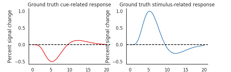
Underlying data-generating model
Because we simulated the data, we know that the event-related responses should exactly follow the canonical Hemodynamic Response Function [1]_are
from nideconv.utils import double_gamma_with_d
import numpy as np

plt.figure(figsize=(8, 2.5))

t = np.linspace(0, 20, 100)
ax1 = plt.subplot(121)
plt.title('Ground truth cue-related response')
plt.plot(t, double_gamma_with_d(t) * -.5,
         color=palette[0])
plt.xlabel('Time since event (s)')
plt.ylabel('Percent signal change')
plt.axhline(0, c='k', ls='--')

plt.subplot(122, sharey=ax1)
plt.title('Ground truth stimulus-related response')
plt.plot(t, double_gamma_with_d(t),
         color=palette[1])
plt.axhline(0, c='k', ls='--')
plt.xlabel('Time since event (s)')
plt.ylabel('Percent signal change')

sns.despine()
Plot simulated data
data.plot(c='k')
sns.despine()

for onset in cue_onsets:
    l1 =plt.axvline(onset, c=palette[0], ymin=.25, ymax=.75)

for onset in stim_onsets:
    l2 =plt.axvline(onset, c=palette[1], ymin=.25, ymax=.75)

plt.legend([l1, l2], ['Cue', 'Stimulus'])
plt.gcf().set_size_inches(10, 4)
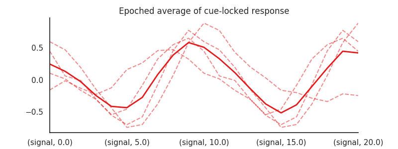
Naive approach: epoched averaging
A simple approach that is appropriate for fast electrphysiological signals like EEG and MEG, but not necessarily fMRI, would be to select little chunks of the time series, corresponding to the onset of the events-of-interest and the subsequent 20 seconds of signal (“epoching”).
We can do such a epoch-analysis using nideconv, by making a ResponseFitter object and using the get_epochs()-function:
rf =nideconv.ResponseFitter(input_signal=data,
                            sample_rate=1)

# Get all the epochs corresponding to cue-onsets for subject 1,
# run 1.
cue_epochs = rf.get_epochs(onsets=onsets.loc['cue'].onset,
                           interval=[0, 20])
Now we have a 4 x 21 DataFrame of epochs, that we can all plot in the same figure:
print(cue_epochs)
cue_epochs.T.plot(c=palette[0], alpha=.5, ls='--', legend=False)
cue_epochs.mean().plot(c=palette[0], lw=2, alpha=1.0)
sns.despine()
plt.xlabel('Time (s)')
plt.title('Epoched average of cue-locked response')
plt.gcf().set_size_inches(8, 3)
Out:
roi      signal                      ...
time       0.0       1.0       2.0   ...      18.0      19.0      20.0
onset                                ...
5     -0.158240 -0.013876 -0.130658  ...  0.548503  0.648452  0.446225
15     0.103284  0.014407 -0.163286  ...  0.454592  0.772234  0.594640
25     0.446225  0.060751 -0.008963  ...  0.070136  0.581173  0.884578
35     0.594640  0.467924  0.194969  ... -0.338853 -0.217950 -0.245611

[4 rows x 21 columns]
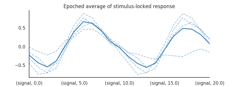
We can do the same for the stimulus-locked responses:
stim_epochs = rf.get_epochs(onsets=onsets.loc['stim'].onset,
                           interval=[0, 20])
stim_epochs.T.plot(c=palette[1], alpha=.5, ls='--', legend=False)
stim_epochs.mean().plot(c=palette[1], lw=2, alpha=1.0)
sns.despine()
plt.xlabel('Time (s)')
plt.title('Epoched average of stimulus-locked response')
plt.gcf().set_size_inches(8, 3)
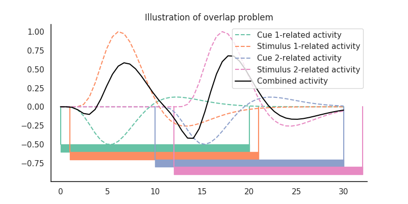
Contamination
As you can see, when we use epoched averaging, both the cue- and stimulus-related response are contaminated by adjacent responses (from both response types). The result is some sinewave-like pattern that has little to do with the data-generating response functions of both cue- and stimulus-related activity
# This is because the event-related responses are overlapping in time:
from nideconv.utils import double_gamma_with_d

t = np.linspace(0, 30)

cue1_response = double_gamma_with_d(t) * -.5
stim1_response = double_gamma_with_d(t-1)

cue2_response = double_gamma_with_d(t-10) * -.5
stim2_response = double_gamma_with_d(t-12)

palette2 = sns.color_palette('Set2')

plt.fill_between([0, 20],  -.5, -.6, color=palette2[0])
plt.plot([[0, 20], [0, 20]], [-.5, 0], color=palette2[0])
plt.fill_between([1, 21],  -.6, -.7, color=palette2[1])
plt.plot([[1, 21], [1, 21]], [-.6, 0], color=palette2[1])
plt.fill_between([10, 30],  -.7, -.8, color=palette2[2])
plt.plot([[10, 30], [10, 30]], [-.7, 0], color=palette2[2])
plt.fill_between([12, 32],  -.8, -.9, color=palette2[3])
plt.plot([[12, 32], [12, 32]], [-.8, 0], color=palette2[3])


plt.plot(t, cue1_response, c=palette2[0], ls='--', label='Cue 1-related activity')
plt.plot(t, stim1_response, c=palette2[1], ls='--', label='Stimulus 1-related activity')

plt.plot(t, cue2_response, c=palette2[2], ls='--', label='Cue 2-related activity')
plt.plot(t, stim2_response, c=palette2[3], ls='--', label='Stimulus 2-related activity')

plt.plot(t, cue1_response + \
            stim1_response + \
            cue2_response + \
            stim2_response,
         c='k', label='Combined activity')
plt.legend()
sns.despine()
plt.gcf().set_size_inches(8, 4)
plt.xlim(-1, 32.5)
plt.title('Illustration of overlap problem')
Solution: the Genera Linear Model
An often-used solution to the “overlap problem” is to assume a linear time-invariant system. This means that you assume that overlapping responses influencing time point \(t\) add up linearly. Assuming this linearity, the deconvolution boils down to solving a linear sytem: every timepoint \(y_t\) from signal \(Y\) is a linear combination of the overlapping responses, modeled by corresponding row of matrix \(X\), \(X_{t,...}\) (note that the design of matrix \(X\) is crucial here but more on that later…). We just need to find the ‘weights’ of the responses \(\beta\).:
We can do this using a General Linear Model (GLM) and its closed-form solution ordinary least-squares (OLS).
This solution is part of the main functionality of nideconv. and can be applied by creating a ResponseFitter-object:
rf =nideconv.ResponseFitter(input_signal=data,
                            sample_rate=1)
To which the events-of-interest can be added as follows:
rf.add_event(event_name='cue',
             onsets=onsets.loc['cue'].onset,
             interval=[0,20])
rf.add_event(event_name='stimulus',
             onsets=onsets.loc['stim'].onset,
             interval=[0,20])
Nideconv aumatically creates a design matrix. By default, it does so using ‘Finite Impulse Response’-regressors (FIR). Each one of these regressors corresponds to a different event and temporal offset. Such a design matrix looks like this:
sns.heatmap(rf.X)
print(rf.X)
Out:
event type confounds           cue  ...      stimulus
covariate  intercept     intercept  ...     intercept
regressor  intercept         fir_0  ...        fir_18        fir_19
time                                ...
0.0              1.0 -1.776357e-17  ... -8.881784e-18 -1.332268e-17
1.0              1.0  4.826947e-17  ... -2.664535e-17 -4.440892e-17
2.0              1.0 -4.440892e-17  ...  4.440892e-17  7.993606e-17
3.0              1.0 -5.329071e-17  ... -1.776357e-17 -1.199041e-16
4.0              1.0 -2.118095e-17  ... -9.025575e-18  0.000000e+00
5.0              1.0  1.000000e+00  ...  3.093534e-17  1.575989e-16
6.0              1.0  2.232659e-17  ... -5.581465e-17 -1.185217e-16
7.0              1.0  1.585169e-17  ... -4.930796e-18 -1.720337e-17
8.0              1.0  6.778588e-18  ... -7.105427e-17  3.392509e-17
9.0              1.0 -7.105427e-17  ... -5.329071e-17  7.105427e-17
10.0             1.0 -4.859750e-18  ...  2.895930e-17  0.000000e+00
11.0             1.0  5.592731e-17  ... -2.254300e-17 -3.006191e-17
12.0             1.0 -6.844479e-17  ...  2.778522e-17 -7.890584e-17
13.0             1.0  3.397045e-17  ...  4.896324e-17  1.757482e-17
14.0             1.0 -5.028678e-17  ...  8.881784e-17 -2.389496e-17
15.0             1.0  1.000000e+00  ... -3.721182e-18 -5.329071e-17
16.0             1.0 -3.778477e-17  ... -1.334069e-17  9.184751e-17
17.0             1.0  1.011971e-17  ...  9.657810e-18 -3.777648e-17
18.0             1.0 -6.931033e-17  ...  4.387637e-17  7.706233e-17
19.0             1.0 -8.881784e-17  ...  0.000000e+00  9.215158e-17
20.0             1.0 -5.162537e-17  ... -2.221190e-17 -3.552714e-17
21.0             1.0 -8.794843e-17  ...  2.086186e-17 -5.928766e-17
22.0             1.0 -2.662462e-17  ... -5.839173e-17  4.416186e-17
23.0             1.0  3.123730e-17  ...  3.732154e-17  7.286403e-17
24.0             1.0  3.763226e-18  ...  1.000000e+00  4.748292e-17
25.0             1.0  1.000000e+00  ... -5.329071e-17  1.000000e+00
26.0             1.0  5.294499e-18  ...  9.016015e-17  0.000000e+00
27.0             1.0  2.584759e-17  ... -1.163986e-17  7.948316e-17
28.0             1.0  6.476414e-17  ... -3.043355e-17 -5.616264e-17
29.0             1.0 -5.443813e-18  ...  6.971763e-18 -1.101554e-16
30.0             1.0 -4.793710e-18  ... -1.421085e-16 -4.724240e-17
31.0             1.0 -3.378831e-17  ...  1.075351e-17 -1.776357e-17
32.0             1.0  7.324020e-17  ... -5.833184e-17  2.331487e-18
33.0             1.0  1.596911e-17  ...  6.006043e-17  2.334715e-17
34.0             1.0  2.431918e-17  ...  1.658620e-17 -6.672890e-17
35.0             1.0  1.000000e+00  ...  1.000000e+00  1.011500e-16
36.0             1.0  2.285811e-17  ... -1.431587e-17  1.000000e+00
37.0             1.0  7.837668e-17  ...  1.517236e-16  0.000000e+00
38.0             1.0 -1.366774e-17  ...  5.183790e-17  1.113862e-16
39.0             1.0  9.552760e-18  ...  4.957410e-18 -1.893770e-17
40.0             1.0 -2.720046e-17  ... -8.881784e-17 -7.646967e-17
41.0             1.0 -8.881784e-17  ...  7.105427e-17  5.329071e-17
42.0             1.0 -4.466079e-18  ... -9.637756e-18 -7.105427e-17
43.0             1.0  1.705257e-17  ... -3.980469e-17 -3.274346e-17
44.0             1.0 -3.366283e-18  ...  1.384605e-17  1.241116e-16
45.0             1.0 -2.989202e-17  ...  4.025400e-18  3.495476e-17
46.0             1.0  4.431898e-17  ...  1.000000e+00  2.199715e-16
47.0             1.0 -1.274637e-16  ...  1.362504e-17  1.000000e+00
48.0             1.0 -4.777595e-18  ...  4.056828e-17  0.000000e+00
49.0             1.0  4.347886e-17  ... -3.391004e-17 -2.334715e-17
50.0             1.0  1.540136e-17  ... -5.251377e-17 -3.047576e-17
51.0             1.0  0.000000e+00  ... -7.105427e-17 -4.995597e-17
52.0             1.0  2.310311e-17  ... -9.275620e-17 -1.421085e-16
53.0             1.0  9.925901e-17  ...  4.160809e-17  9.673688e-17
54.0             1.0  6.037837e-17  ...  2.200937e-17  2.644305e-17
55.0             1.0 -5.236773e-17  ...  1.389141e-16 -1.256192e-17
56.0             1.0  2.483597e-17  ... -8.881784e-17  4.297320e-17
57.0             1.0 -1.776357e-17  ...  1.000000e+00  5.329071e-17
58.0             1.0  2.733866e-17  ...  1.368792e-18  1.000000e+00
59.0             1.0 -1.968355e-17  ... -2.763133e-17  0.000000e+00

[60 rows x 41 columns]
(Note the hierarchical columns (event type / covariate / regressor) on the regressors)
Now we can solve this linear system using ordinary least squares:
rf.fit()
print(rf.betas)
Out:
signal
event type covariate regressor
confounds  intercept intercept  0.023102
cue        intercept fir_0     -0.100649
                     fir_1     -0.063218
                     fir_2      0.060717
                     fir_3     -0.205428
                     fir_4     -0.320793
                     fir_5     -0.500031
                     fir_6     -0.465807
                     fir_7     -0.436244
                     fir_8     -0.217273
                     fir_9     -0.149503
                     fir_10     0.123602
                     fir_11     0.121397
                     fir_12     0.025211
                     fir_13     0.162086
                     fir_14     0.105873
                     fir_15     0.132055
                     fir_16     0.056222
                     fir_17     0.130353
                     fir_18     0.036380
                     fir_19     0.175794
stimulus   intercept fir_0      0.095643
                     fir_1     -0.093245
                     fir_2      0.076270
                     fir_3      0.272010
                     fir_4      0.706539
                     fir_5      0.827825
                     fir_6      0.989700
                     fir_7      0.763656
                     fir_8      0.519356
                     fir_9      0.137110
                     fir_10    -0.000634
                     fir_11    -0.248265
                     fir_12    -0.157455
                     fir_13    -0.318611
                     fir_14    -0.300280
                     fir_15    -0.347443
                     fir_16    -0.147481
                     fir_17    -0.171133
                     fir_18    -0.068836
                     fir_19    -0.016540
Importantly, with nideconv it is also very easy to ‘convert` these beta-estimates to the found event-related time courses, at a higher temporal resolution:
tc =rf.get_timecourses()
print(tc)
Out:
signal
event type covariate time
cue        intercept 0.00  -0.100649
                     0.05  -0.100649
                     0.10  -0.100649
                     0.15  -0.100649
                     0.20  -0.100649
                     0.25  -0.100649
                     0.30  -0.100649
                     0.35  -0.100649
                     0.40  -0.100649
                     0.45  -0.100649
                     0.50  -0.100649
                     0.55  -0.063218
                     0.60  -0.063218
                     0.65  -0.063218
                     0.70  -0.063218
                     0.75  -0.063218
                     0.80  -0.063218
                     0.85  -0.063218
                     0.90  -0.063218
                     0.95  -0.063218
                     1.00  -0.063218
                     1.05  -0.063218
                     1.10  -0.063218
                     1.15  -0.063218
                     1.20  -0.063218
                     1.25  -0.063218
                     1.30  -0.063218
                     1.35  -0.063218
                     1.40  -0.063218
                     1.45  -0.063218
...                              ...
stimulus   intercept 18.50 -0.068836
                     18.55 -0.016540
                     18.60 -0.016540
                     18.65 -0.016540
                     18.70 -0.016540
                     18.75 -0.016540
                     18.80 -0.016540
                     18.85 -0.016540
                     18.90 -0.016540
                     18.95 -0.016540
                     19.00 -0.016540
                     19.05 -0.016540
                     19.10 -0.016540
                     19.15 -0.016540
                     19.20 -0.016540
                     19.25 -0.016540
                     19.30 -0.016540
                     19.35 -0.016540
                     19.40 -0.016540
                     19.45 -0.016540
                     19.50 -0.016540
                     19.55 -0.016540
                     19.60 -0.016540
                     19.65 -0.016540
                     19.70 -0.016540
                     19.75 -0.016540
                     19.80 -0.016540
                     19.85 -0.016540
                     19.90 -0.016540
                     19.95 -0.016540

[800 rows x 1 columns]
as well as plot these responses…
sns.set_palette(palette)
rf.plot_timecourses()
plt.suptitle('Linear deconvolution using GLM and FIR')
plt.title('')
plt.legend()
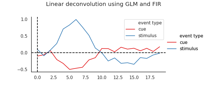
As you can see, these estimated responses are much closer to the original data-generating functions we were looking for.
Cleary, the linear deconvolution approach allows us to very quickly and effectively ‘decontaminate’ overlapping responses. Have a look at the next section () for more theory and plots on the selection of appropriate basis functions.
References
| [1] | Glover, G. H. (1999). Deconvolution of impulse response in |
event-related BOLD fMRI. NeuroImage, 9(4), 416–429.
Total running time of the script: ( 0 minutes 2.383 seconds)